Don't Say "There Must Be Something Common, Or They Would Not Be Called 'Games'"

1.0 Introduction
Von Neumann and Morgenstern posed a mathematical problem in 1944: Does every game have a solution, where a solution is defined in their sense? W. F. Lucas solved this problem in 1967. Not all games have such a solution. (It is known that such a solution need not be unique. In fact, the solution to the three person game I use below to illustrate the Von Neumann and Morgenstern solution is not unique.)

I may sometime in the future try to explain the game with ten players Lucas presents as a counterexample, assuming I can grasp it better than I do now. With this post, I try to explain some concepts of cooperative game theory so as to have this post for reference when and if I do. The Nash equilibrium and refinements are notions from the different theory of non-cooperative game theory.

2.0 Definition of a Game
Roughly, a game is specified by:

• The number of players
• The strategies available for each player
• The payoffs to each player for each combination of player strategies

How a strategy is described depends on the specification of the game - whether it is in extensive form, normal form, or characteristic function form. Von Neumann and Morgenstern hoped that all three forms would be equivalent, with less data needing to be specified in the later forms in this series. This hope has arguably not worked out.

2.1 Extensive Form
A game in extensive form is specified as a tree. This is most easily seen for board games, like backgammon or chess. Each node in the tree is a board position, with the root of the tree corresponding to the initial position.

The specification of a node includes which player is to move next, as well as the board position. Each possible move the player whose turn it is can make is shown by a link leading from the node to a node for the board position after that choice of a move. Random moves are specified as moves made by a fictitious player, who might be named "Mother Nature". The roll of a pair of dice or the deal of a randomly selected card are examples of random moves. With a random move, the probability of each move is specified along the line connecting one node to another. Since a move by an actual player is freely chosen, the probabilities of any move by an actual player are not specified in the specification of a game.

The above description of the specification of a game cannot yet handle games like poker. In poker, not every player knows every card that is dealt. Von Neumann and Morgenstern introduce the concept of "information sets" to allow one to specify that, for instance, a player only knows all the cards in his hands and, perhaps, some of the cards in the other players' hands. An information set at a node, specifies for the player whose turn it is, which of the previous choices of moves in the game he has knowledge of. That is, an information set is a subset of the set of links in the tree leading from the initial position to the current node position. Since some of these moves were random, this specification allows for the dealing of hands of cards, for example.

The final element in this specification of a game occurs at the leaves of the tree. These are the final positions in the games. Leaves have assigned the values of the payouts to each player in the game.

It is easy to see how to define a player's strategy with this specification of a game. A strategy states the player's choice of a move at each node in the game denoting a position in which it is the player's move. A play of the game consists of each player specifying their strategy and the random selection of a choice from the specified probability distributions at each node at which a random move is chosen. These strategies and the random moves determine the leaf at which the game terminates. And one can then see the payouts to all players for the play.

One can get rid of the randomness, in some sense, by considering an infinite number of plays of the game for each combination of players' strategies. This will result in a probability distribution for payouts. The assumption is that each player is interested in the expected value, that is, the mean payout, to be calculated from this probability distribution. (All these descriptions of calculations have abstracted from time and space computational constraints.)

2.2 Normal Form
One abstracts from the sequence of moves and from random moves in specifying a game in normal form. The extensive form allows for the definition of strategies for each player, and each strategy can be assigned an arbitrary label. A game in normal form consists of a grid or table. A player's strategies are listed along one dimension of the table, and each dimension corresponds to a player. Each entry in the table consists of a ordered tuple, where the elements of the tuple are the expected payouts to the players for the specified combination of strategies.

Table 1 shows a simple example - the children's game, "Rock, Paper, Scissors." The rules specify the winner. Rock crushes scissors, scissors cut paper, and paper covers rock. This is a two-person zero-sum game. The payouts are shown in the table for the player whose strategies are listed for each row to the left. The payouts to the column player are, in this case, the additive inverse of the table entries.

Table 1: Rock, Paper, Scissors

	Rock	Scissors	Paper
Rock	0	+1	-1
Scissors	-1	0	+1
Paper	+1	-1	0

By symmetry, no pure strategy in Rock, Paper, Scissors is better than any other. A mixed strategy is formed for a player by assigning probabilities to each of that player's pure strategies. Probabilities due to states of nature are removed in the analysis of games by taking mathematical expectations. But probabilities reappear from rational strategization. I also found interesting Von Neumann and Morgenstern's analysis of an idealized form of poker. One wants one's bluffs to be called in bluffing on occasion so that players will be willing to add more to the pot when one raises on a good hand.

Each player's best mixed strategy in a two-person zero-sum game can be found by solving a Linear Program (LP). Let p₁, p₂, and p₃ be the probabilities that the row player in Table 1 chooses strategies Rock, Scissors, and Paper, respectively. The value of the game to the row player is v. The row player's LP is:

Choose p₁, p₂, p₃, v
To Maximize v
Such that
-p₂ + p₃ ≥ v
p₁ - p₃ ≥ v
-p₁ + p₂ ≥ v
p₁ + p₂ + p₃ = 1
p₁ ≥ 0, p₂ ≥ 0, p₃ ≥ 0

The interest of the column player is to minimize the payout to the row player. The left-hand sides of the first three constraints show the expected value to the row player when the column player plays Rock, Scissors, and Paper, respectively. That is, the coefficients by which the probabilities are multiplied in these constraints come from the columns in Table 1. Given knowledge of the solution probabilities, the column player can guarantee the value of the game does not exceed these expected values by choosing the corresponding column strategy. That is, the column player chooses a pure strategy to minimize the expected payout to the row player.

The column player's LP is the dual of the above LP. As a corollary of duality theory in Linear Programming, a minimax solution exists for all two-person zero-sum games. This existence is needed for the definition of the characteristic function form of a game.

2.3 Characteristic Function Form
The characteristic function form of a game is defined in terms of coalitions of players. An n-person game is reduced to a two-person game, where the "players" consist of a coalition of true players and the remaining players outside the coalition. The characteristic function for a game is the value of the corresponding two-person zero-sum game for each coalition of players. The characteristic function form of the game specifies the characteristic function.

As an illustration, Von Neumann and Morgenstern specify the three-person game in Table 2. In this game, coalitions of exactly two people win a unit.

Table 2: Canonical Three Person Game

Coalition	Value
{ }	v( { } ) = 0
{1}	v( {1} ) = -1
{2}	v( {2} ) = -1
{3}	v( {3} ) = -1
{1, 2}	v( {1, 2} ) = 1
{1, 3}	v( {1, 3} ) = 1
{2, 3}	v( {2, 3} ) = 1
{1, 2, 3}	v( {1, 2, 3} ) = 0

3.0 A Solution Concept

Definition: An imputation for an n-person game is an n-tuple (a₁, a₂, ..., a_n) such that:

• For all players i, the payout to that player in the imputation does not fall below the amount that that player can obtain without the cooperation of any other player. That is, a_i ≥ v( {i} ).
• The total in the imputation of the payouts over all players is the payout v( {1, 2, ..., n} ) to the coalition consisting of all players.

Definition: An imputation a = (a₁, a₂, ..., a_n) dominates another imputation b = (b₁, b₂, ..., b_n) if and only if there exists a set of players S such that:

• S is a subset of {1, 2, ..., n}
• S is not empty
• The total in the imputation a of the payouts over all players in S does not exceed the payout v( S ) to the coalition consisting of those players
• For all players i in S, the payouts a_i in a strictly exceed the payouts b_i in b

Definition: A set of imputations is a solution (also known as a Von Neumann and Morgenstern solution or a stable set solution) to a game with characteristic function v( ) if and only if:

• No imputation in the solution is dominated by another imputation in the solution
• All imputations outside the solution are dominated by some imputation in the solution

Notice that an imputation in a stable set solution can be dominated by some imputation outside the solution. The following set of three imputations is a solution to the three-person zero-sum game in Table 2:

{(-1, 1/2, 1/2), (1/2, -1, 1/2), (1/2, 1/2, -1)}

This solution is constructed by considering all two-person coalitions. In each imputation in the solution, the payouts to the winning coalition are evenly divided.

The above is not the only solution to this game. An uncountably infinite number of solutions exist. Another solution is the following uncountable set of imputations:

{(a, 1 - a, -1) | -1 ≤ a ≤ 2}

This solution can be understood in at least two ways:

• Player 3 is being discriminated against.
• The above is a solution to the two-person, non-constant game with the characteristic function in Table 3. A fictitious third player has been appended to allow the game to be analyzed as a three-person zero-sum game.

Von Neumann and Morgenstern present both interpretations.

Table 3: A Two-Person Game With Variable Sum

Coalition	Value
{ }	v( { } ) = 0
{1}	v( {1} ) = -1
{2}	v( {2} ) = -1
{1, 2}	v( {1, 2} ) = 1

The above has defined the Von Neumann and Morgenstern solution to a game. Mathematicians have defined at least one other solution concept to a cooperative game, the core, in which no imputation in the solution set is dominated by any other imputation. I'm not sure I consider the Shapley value as a solution concept, although it does have the structure, I guess, of an imputation.

References

• W. F. Lucas, "A Game With No Solution", Bulletin of the American Mathematical Society, V. 74, N. 2 (March 1968): 237-239
• John von Neumann and Oskar Morgenstern, Theory of Games and Economic Behavior, Princeton University Press (1944, 1947, 1953)

Negative Price Wicksell Effect, Positive Real Wicksell Effect

1.0 Introduction
I have previously suggested a taxonomy of Wicksell effects. This post presents an example with:

• The cost-minimizing technique varying continuously along the so-called factor-price frontier
• Negative price Wicksell effects
• Positive real Wicksell effects
• Price Wicksell effects greater in magnitude than real Wicksell effects.

This example is due to Saverio M. Fratini ("Reswitching and Decreasing Demand for Capital").

2.0 Technology
Suppose technology consists of a continuum of techniques indexed by the parameter θ, where θ is a real number restricted to the interval [0, 1]:

0 ≤ θ ≤ 1

Each technique consists of the three Constant-Returns-to-Scale processes in Table 1. No commodity is basic, in Sraffa's sense, in any technique in this technology. In the first process in a technique, θ-grade iron is produced directly from unassisted labor. In the second process, labor transforms the θ-grade iron into θ-grade steel. Finally, in the third process, labor transforms θ-grade steel into corn, the consumption good in the model. All processes take a year to complete, and all processes totally use up their input.

Table 1: The Technique Indexed by θ

Inputs	Industry Sector
	θ-Grade Iron	θ-Grade Steel	Corn
Labor (Person-Yrs)	1/(1 + θ)	θ	3/(1 + θ)
Iron (Tons)	0	1	0
Steel (Tons)	0	0	1
Corn (Bushels)	0	0	0
Output	1 Ton	1 Ton	1 Bushel

Capital goods are specific in their uses in this example. θ₁-grade steel cannot be made out of θ₂-grade iron when θ₁ ≠ θ₂.

3.0 Stationary-State Quantity Flows
Suppose in Table 1 that:

• The first process is used to produce (1 + θ)/(4 + θ + θ²) tons of θ-grade iron
• The second process is used to produce (1 + θ)/(4 + θ + θ²) tons of θ-grade steel
• The third process is used to produce (1 + θ)/(4 + θ + θ²) bushels corn

Then one person-year would be employed over these three processes. Capital goods would consist of (1 + θ)/(4 + θ + θ²) tons of θ-grade iron and (1 + θ)/(4 + θ + θ²) tons of θ-grade steel. The capital goods would be used up throughout the latter two sectors, but reproduced at the end of the year. Net output would consist of (1 + θ)/(4 + θ + θ²) bushels corn per person-year.

4.0 Prices
Given the technique, stationary state prices must satisfy the following three equations:

[1/(1 + θ)] w = p₁

p₁(1 + r) + θ w = p₂

p₂(1 + r) + [3/(1 + θ)] w = 1

where:

• p₁ is the price of a ton θ-grade iron;
• p₂ is the price of a ton θ-grade steel;
• w is the wage;
• r is the rate of profits.

A bushel corn is the numeraire. The above equations embody the assumption that labor is paid at the end of the year.

The above is a system of three equations in four unknowns, given the technique. It is a linear system, given the rate of profits. The solution in terms of the rate of profits is easily found. The so-called factor-price curve for a technique is:

w(r, θ) = (1 + θ)/[3 + θ(1 + θ)(1 + r) + (1 + r)²]

The price of a ton θ-grade iron is:

p₁(r, θ) = 1/[3 + θ(1 + θ)(1 + r) + (1 + r)²]

The price of a ton θ-grade steel is:

p₂(r, θ) = [(1 + r) + θ(1 + θ)]/[3 + θ(1 + θ)(1 + r) + (1 + r)²]

Given the technique and the rate of profits, these prices can be used to evaluate the value of the capital goods used in a stationary state.

5.0 The Cost-Minimizing Technique
The optimal technique to use at any given rate of profits maximizes the wage. The first-order condition for such maximization is found by equating the derivative of the factor-price curve to zero:

dw/dθ = 0

Or:

3 + θ(1 + θ)(1 + r) + (1 + r)² - (1 + θ)(1 + 2θ)(1 + r) = 0

For 0 ≤ r ≤ 2, the cost-minimizing technique is then:

θ(r) = {[3 + (1 + r)²]/(1 + r)}^1/2 - 1

For r > 2, a corner solution is found:

θ(r) = 1

Figure 1 illustrates the cost-minimizing technique.

Figure 1: The Choice of Technique

The graph in Figure 1 reaches a minimum at a rate of profits of (3^1/2 - 1). For (12^1/4 - 1) < θ < 1, two rate of profits have the corresponding cost-minimizing technique indexed by the given value of θ. In other words, this is an example of reswitching.

The index for the cost-minimizing technique can be plugged into the factor price curve for the technique to which it corresponds at a given rate of profits. Figure 2 displays the resulting so-called factor price frontier. The index θ varies continuously for 0 ≤ r ≤ 200% in Figure 2. As the rate of profits increases without bound, the frontier approaches a wage of zero.

Figure 2: The Factor-Price Frontier

6.0 Capital and Labor "Markets"
Fratini’s notes that this is a reswitching example in which the capital market initially appears to be in accord with out-dated neoclassical intuition. The above analysis has shown how to find physical quantities of capital goods per worker, how to evaluate them at equilibrium prices, and how to find net output per worker. Figure 3 shows the resulting plot of the value of capital per unit output. Fratini looks at the value of capital per worker instead. Either curve is continuous and downward-sloping. The regions above and below the rate of profits of (3^1/2 - 1) appear qualitatively similar and visually indistinguishable. This curve might be said to be a downward-sloping demand function for capital.

Figure 3: The Capital Market

The analogous curve looks very different for the labor market (Figure 4). The region with a positive Wicksell effect is a region with a high rate of profits and thus a low real wage. The demand function for labor might be said to be upward-sloping in the region with a positive real Wicksell effect.

Figure 4: The Labor Market

7.0 Conclusion
The example makes Fratini’s point. The shape of the relationship between the value of capital, either per worker or per unit output, and the rate of profits is not necessarily a good indicator of the presence of reswitching or reverse capital-deepening.

Simple and Expanded Reproduction

1.0 Introduction
This post presents a model in which a capitalist economy smoothly reproduces itself. The purpose of such a model is not to predict that capitalist economies will converge to some such path as illustrated in the model. Rather, the model provides a basis for the analysis of where things can go wrong.

This sort of model has a long history. My exposition is close to Marx (1956), with the difference that Marx sets out the conditions of simple and expanded production in terms of labor values, not in terms of prices of production. Rosa Luxemburg (1951) and Michal Kalecki (1969) used Marx's department break-down to develop a Keynes-like model of the long run and the short run. Shigeto Tsuru (1942) apparently exposed this model to english-speaking academics when few were looking at Marx's analysis. Joan Robinson (1962) drew on these ideas, among others, in her models of metallic ages. Goodwin's generalization (1949) of Keynes to a multisectorial model and Pasinetti's (1981, 1993) analyses of vertically integrated sectors also seem to me to bear family resemblances to this model. Doubtless, my references could be extended in many directions.

Table 1: Definition of Variables

Variable	Definition
	The person-years of labor hired per unit output (e.g., ton steel) in the first sector.
	The person-years of labor hired per unit output (e.g., bushel corn) in the second sector.
	The capital goods used up per unit output in the first (steel-producing) sector.
	The capital goods used up per unit output in the second (corn-producing) sector.
	The price of unit output in the first sector.
	The price of unit output in the second sector.
	The rate of profits.
	The savings rate out of profits.
	The wage, that is, the price of hiring a person-year.
	The number of units (tons steel) produced in the first sector.
	The number of units (bushels corn) produced in the second sector.

2.0 Two Departments
This model considers a capitalist economy with no government and no foreign trade. The outputs of this economy are grouped into two great departments. In the first department, capitalists direct workers to produce means of production (also known as capital goods) with the means of production in that department. In the second department, the workers are directed to produce means of consumption (also known as consumption goods) with the means of production in that department.

For ease of exposition, I make certain additional simplifying assumptions. The workers consume all of their wages. Only the capitalists save, and they save only in the case of expanded reproduction. All capital is circulating capital. That is, there is no fixed capital, such as long-lived machinery. In other words, all capital goods are totally used up each year in producing the yearly output. No technological innovations are introduced.

I think introducing technological innovations and fixed capital makes the possibility of smooth reproduction more incredible. A govenrment can be introduced as a third department, or perhaps by dividing government output among the two departments shown. Foreign trade introduces the possibility of correcting imbalances in domestic demand from outside the domestic economy. But then one could recast the model as of the world economy.

3.0 Prices
A necessary condition for smooth reproduction of a competitive capitalist economy is that the same rate of profit be made in all departments. Otherwise, some capitalists are finding that the expectations on which investments were made are being unfulfilled. They would want to have contracted some departments and expanded others. I also impose the condition that spot prices remain stationary. Equations 1 and 2 express these conditions:

(1)

(2)

I suppose one could put time indices on the prices in Equations 1 and 2, thereby defining a dynamic system for prices. Suppose distribution and the ratios of physical quantity flows remain unchanged year after year. Then the steady-state prices expressed in Equations 1 and 2 (without time indices) would be a limit point of the dynamic process so defined. It is this caveat, I think, that allows me to ignore that constant prices are, perhaps, not a necessary condition for smooth reproduction.

Table 2: Values of Outputs By Department and Distribution

Department	Capital	Wages	Profits
Capital Goods
Consumption Commodities

4.0 In Balance
4.1 Simple Reproduction
The economy is in simple reproduction when it is replicated on the same scale year after year. A necessary condition for an economy in simple reproduction is that the production of capital goods each year be equal to the capital goods used up each year. In the model shown here, the value of the capital goods used up each year must equal the value of the output of the first department:

(3)

Equation 3 can be simplified:

(4)

Equation 4 is easily summarized in words. It states that the value of capital goods demanded from the second department matches the demand for consumption goods from the first department. In a sense, Equation 4 is a generalization of Keynes' idea of effective demand. The condition that all workers looking for a job are able to find one at the going wage is a separate condition, not stated here. In a sense, this model generalizes Keynes' theory, in some sense, to the long-run.

An alternate method of deriving Equation 4 is available. Start from the equation of the value of total demand for consumption goods and the value of the output of the department producing consumption goods. This condition, when simplified, also yields Equation 4.

4.2 Expanded Reproduction
The economy experiences expanded reproduction when it consistently expands each year. In this case, the demand for capital goods from the second department includes the savings of the capitalists receiving profits from that department. Likewise, the demand for consumption goods from the first department excludes the savings of the capitalists in that department. Observing these qualifications, it is easy to mathematically express the condition that the demand for capital goods from the second department match the demand for consumption goods from the first department:

(5)

Or:

(6)

Focus on the left-hand side of Equation 6. Is it apparent that the rate of growth in expanded reproduction in this model is the product of the capitalists' saving propensity and the rate of profit? In other words, the rate of profit along a warranted growth path is the quotient of the rate of growth and the saving propensity of the capitalists. So this model points to a Post Keynesian theory of distribution.

5.0 Conclusion
In the model, capitalists independently decide on what department to enter, and how much to produce in that department. A collective result of those decisions is the total output of each department. For those decisions to be validated, the value of consumer goods demanded by workers and capitalists in the department producing capital goods must match the value of capital goods demanded by the capitalists in the department producing consumption goods.

The model is silent on how such an equality can come about. Supply and demand seems like an inadequate answer to me.

References

• Richard M. Goodwin (1949). "The Multiplier as Matrix", Economic Journal, V. 59, N. 236 (Dec.): 537-555
• M. Kalecki (1969). Theory of Economic Dynamics: An Essay on Cyclical and Long-Run Changes in Capitalist Economy, Second Edition, Augustus M. Kelly
• Rosa Luxemburg (1951). The Accumulation of Capital (Trans. by Agnes Schwarzschild), Yale University Press
• Karl Marx (1956). Capital, Volume 2, Progress Publishers
• Luigi L. Pasinetti (1981). Structural Change and Economic Growth: A Theoretical Essay on the Dynamics of the Wealth of Nations, Cambridge University Press
• Luigi L. Pasinetti (1993). Structural Economic Dynamics: A Theory of the Economic Consequences of Human Learning, Cambridge University Press
• Joan Robinson (1962). Essays in the Theory of Economic Growth, Macmillan
• Shigeto Tsuru (1942). "On Reproduction Schemes", Appendix A in Paul Sweezy's The Theory of Capitalist Development, Monthly Review Press [This reference I haven't read]

An Indeterminate Two-Person Zero-Sum Game With Perfect Information

1.0 Introduction
I have stumbled upon some odd mathematics, some mathematics that I have not validated. Consider the claim that all two-person zero-sum games with perfect information have a value. Apparently, this claim is inconsistent with the Axiom of Choice, an axiom in set theory. This inconsistency is shown by the Banach-Mazur game and its variants. I guess it is essential to this demonstration that these games have a potentially countable infinite number of moves.

I don't know that this demonstration is as important for economics as, for instance, W. F. Lucas' example of a cooperative game without an equilibrium.

A game has perfect information if the results of all moves prior to any given move are known to all players. Simple examples of games with imperfect information are card games in which the deal gives a player a hand which only he knows. A two-person zero-sum game is determinate if one can prove either (1) the first player wins some definite amount, (2) the second player wins some definite amount, or (3) the game is a draw. Chess is a determinate game, although it is in practice impossible to expand the tree enough to determine its value.

2.0 A Game
I steal this example from a Usenet post by Herman Rubin.

The game is fully specified by the rules and by defining a set C, where C is a given subset of the real numbers between 0 and 1, inclusive. The two players alternatively select the successive binary digits of the base-two expansion of a number within the interval [0, 1].

In other words, consider the number:

(1/2) x₁ + (1/4) x₂ + (1/8) x₃ + (1/16) x₄ + ...

where, for all i, x_i is in {0, 1}. The first player chooses the binary digits with the odd indices, and the second player chooses the binary digits with the even indices. But they take turns and go in order.

The game ends with the second player paying the first player a unit when it is guaranteed that any further expansion will result in a number within C. The game ends with the second player winning a unit payment from the first player when it is guaranteed that any further expansion will result in a number in the complement of C.

A simple example is C = [0.5, 1]. The first player wins in this case. A more complicated game arises when C is the set of all irrational numbers in the unit interval. I gather this game is determinate, but I don't see offhand who wins. Finally, consider a set C that does not have a Lebesque measure. (The Axiom of Choice is necessary for the definition of such a set.) I gather that in this case, the game is not determinate. Nobody can tell a priori who will win.

Militant Voting

This post illustrates a phenomenon that is a possibility in pairwise voting. Consider a constituency of 30 voters deciding among six candidates for a given vacancy. (I take this example from Donald Saari.) Table 1 describes the preferences of these voters. For example, the first row shows that ten voters prefer Anne to Barb, and Barb to Carol, and so on.) The voters are asked to choose between successive pairs of candidates, as shown in Figure 1. In the first election, Debra defeats Elaine. But Carol defeats Debra in the next choice. And so on, until Flicka is the only choice standing, after a landslide victory. It seems that clearly Flicka is the consensus choice. Strangely enough, though, every voter prefers Carol, Debra, and Elaine to Flicka. The voting system doesn’t seem to allow for a true expression of the preferences of the members of the electorate.

Table 1: Voter Preferences

Number	Preference Ranking
10	A > B > C > D > E > F
10	B > C > D > E > F > A
10	C > D > E > F > A > B

Figure 1: Pairwise Elections in Example

Militant was a Trotskyite tendency practicing entryism within the British Labour Party. They seemed to have figured out how to use party discipline to have their way in Liverpool in the early 1980s:

"All political parties on the Monday before the Council meeting on a Wednesday, have a caucus meeting to decide the line of approach at the Council. The agenda for the meeting comes out on a Friday. The ten or twelve Militant members ... meet on either the Friday or the Saturday and go through the agenda to look for important policy decisions and for important vacancies. They then have a meeting with the broad left of the Labour group on Sunday morning at Pirrie Labour Club ... those Militants turn up in their full strength. There are generally about twenty people and the ten or eleven Militants there. They carry the majority vote there that commits the broad left for the meeting of the Labour group. On the Monday night at the Labour group meeting of forty-two members the commitment that Militant have made themselves, plus other people they've taken along at the meeting on Sunday morning, gives them a majority. ... so you find that of forty-two Labour councilors, ten Militants control the policy of the Labour group." -- Eddie Roderick, as quoted by Michael Crick

Crick says, "Roderick's analysis may be a rather simplified version." At any rate, Figure 2 illustrates how the Council seems to have made their decisions. Figures 1 and 2 look quite similar. Maybe Saari’s math describes more than a theoretical possibility.

Figure 1: Pairwise Voting on the Liverpool City Council

References

• Michael Crick (1984). Militant, Faber and Faber
• Donald G. Saari (2004). "Geometry of Chaotic and Stable Discussion", American Mathematical Monthly, V. 111, N. 5: 377-393

For Whatever Can Walk - It Must Walk Once More

1.0 Introduction
This post presents a simple macroeconomic model that combines trend and cycle. It presents some possible aspects of economic growth and business cycles. This model has some features that I find objectionable, but I find it interesting nonetheless. It is a non-linear model of dynamics presenting a formalization of some ideas to be found in Marx's Capital. And it is a model that does not impose equilibrium, but allows for the stability of equilibrium to be analyzed.

2.0 Technology
Assume a Leontief (fixed coefficients) production function:

q = min(a l, k/σ)

where q is gross output, l is the labor employed, k is the value of capital, a is labor productivity, and σ is the capital-output ratio. Both constraints in the production function are always met with equality:

l = q/a

σ = k/q

The capital stock is always employed, but sometimes employment can fall short of the entire labor force, as explained below.

The capital stock depreciates at a rate of 100 δ percent. That is, output can either be consumed or added to a capital stock that experiences a force of mortality of δ. Technical progress is disembodied, and labor productivity increases at a constant rate:

a = a₀ exp( α t )

The labor force also grows at a constant rate:

n = n₀ exp( β t)

where n is the labor supply. Hence, v is the employment rate, where the employment rate is defined as follow:

v = l/n

When v is unity, the labor force is fully employed. v ranges from (a subinterval of) zero to unity in this model.

3.0 Wages, Profits, Investment
Let w be the wage rate. Then (w l) or (w q/a) are total wages. Define u to be the workers share of the gross product:

u = w/a

Then (1 - u) is the capitalists' share of the product. Assume that wages are entirely consumed and that a fixed proportion of profits are saved and invested:

dk/dt = s (1 - u) q - δ k

where s is the savings rate out of profits.

Finally, assume that the rate of growth of wages is a (linear) increasing function of the employment rate:

(1/w) dw/dt = - γ + ρ v

The above equation could also be written as:

(1/w) dw/dt = ρ [v - (γ/ρ) ]

In words, wages grow faster in a tight labor market. The marginal productivity of labor is beside the point in this model.

4.0 Derivation of the Model
The rate of growth of the employment rate is the difference between the rate of growth of employment and the rate of growth of the labor force:

(1/v) dv/dt = (1/l) dl/dt - β

By similar manipulations, one can show that the rate of growth of employment is the difference between the rate of growth of output and the rate of growth of productivity:

(1/l) dl/dt = (1/q) dq/dt - α

Combining these two equations yields an equation relating the rate of growth of the employment rate to the rate of growth in output:

(1/v) dv/dt = (1/q) dq/dt - (α + β)

The derivation of the following equation from the definition of the capital-output ratio and the equation for the rate of change in the value of capital is simpler:

(1/q) dq/dt = (1 - u) s/σ - δ

Hence,

(1/v) dv/dt = (1 - u)(s/σ) - (α + β + δ)

The rate of growth of workers' share in gross ouput is the difference between the rate of growth of wages and the rate of growth of productivity:

(1/u) du/dt = (1/w) dw/dt - α

Substitute from the postulated relation between the rate of growth in wages and the employment rate:

(1/u) du/dt = ρ v - (α + γ)

The following pair of equations, the fundamental equations of this model, restate equations derived above:

dv/dt = (s/σ - α - β - δ) v - (s/σ) u v

du/dt = -(α + γ) u + ρ u v

Here's the cool part - this is the Lotka-Volterra predator-prey model. It is a canonical non-linear dynamical system used to model, say, lynx and rabbits.

5.0 Solution of the Model
For what its worth, a trajectory in phase space has the equation:

(u^ν₁) exp(- θ₁ u) = H(v^{- ν₂}) exp(θ₂ v)

where

θ₁ = s/σ

θ₂ = ρ

ν₁ = s/σ - (α + β + δ)

ν₂ = (α + γ)

and H is an arbitrary integrating constant. All these trajectories consist of cycles, as illustrated in Figure 1. The limit point around which these trajectories cycle is given by:

u* = ν₁/θ₁

v* = ν₂/θ₂ = (α + γ)/ρ

(The origin in phase space is also a limit point; the origin has the stability of a saddle-point.)

Figure 1: Phase Space

Figure 2: A Trajectory

6.0 Discussion
I think it interesting to note that the rate of growth of wages at the limit point is positive due to growth in productivity; in fact, the rate of growth of wages at the limit point is equal to the rate of growth in productivity. If productivity did not grow, if the labor force were stationary, and if there were no depreciation, wages would consume the entire product at the limit point; the capitalists would receive no profits.

A single cycle can easily be described in intutitive terms. Start with low unemployment. Wages will increase as a share in output. Consequently, saving and investment will decline. The growth of output will slow. Eventually, the "reserve army of the unemployed" will be recreated. Wages will decrease as a share in output, although they may still be increasing in absolute terms. Eventually, investment will pick back up. When the growth of output exceeds the growth in productivity by more than the growth of the labor force, the employment rate will increase.

Clearly, this model can reproduce a qualitative resemblance to some empirical properties of some economic time series. If one plots empirical data in the illustrated phase space, one may see a suggestion of motion in the indicated directions, but one will not find a single cycle. Perhaps shocks change the parameters of the model on some occasions. Or perhaps important considerations are not embodied in the model. This model is Classical in important respects, where I mean by "Classical" to refer to the economics of Smith and Ricardo. Richard Goodwin, the inventor of this model, has done important work attempting to integrate this model with Keynesian and Schumpeterian themes.

References
There was a conference in Sienna a number of years back devoted to this model. There's also discussion of this model in a Festschrift volume devoted to Richard Goodwin.

• Richard Goodwin, "A Growth Cycle," in Socialism, Capitalism, & Economic Growth: Essays Presented to Maurice Dobb, (edited by C. H. Feinstein), Cambridge University Press, 1967.
• Richard Goodwin, Chaotic Economic Dynamics, Oxford University Press, 1990.
• Paul Ormerod, The Death of Economics, St. Martins, 1994.

Update: Serena Sordi has a recent generalization of this model to four dimensions, presented at a sort of festschrift for Barkley Rosser, Jr.

Chaotic Cobwebs (Part 1 1/2)

5.0 Return to a Special Case

This post continues the examination of a cobweb cycle with a non-linear demand curve. In this part, I talk again about the special case examined in Section 3 of that previous post. In that case, the parameters b and e of the model are zero. Furthermore, I continue to assume c is 3/5 and d is 21/20. Figure 6 shows attracting limiting behavior for a whole range of the parameter a. The abscissa in this graph is a, with a set to unity at the right edge. The ordinate is the limiting values of the normalized quantity, Q(t). As I point out towards the right, a two-period cycle shows up on the graph as a plot of two values of the ordinate for the value of a for which that cycle is generated. One can see the period-doubling scenario leading to chaos as one moves to the left on the graph. By the way, this figure is a fractal, repeating on an infinite number of scales. It has both qualitative and quantitative universal features for a certain family of one-dimensional maps (for example, characterized by the Feigenbaum constant).

Figure 6: Structural Dynamics of a Special Case

6.0 An Economically Relevant Special Case

The case above has both demand and supply functions through the origin in the quantity-price space. I want to consider a case in which the demand curves intersects the price axis at a strictly positive price and slopes downward in the first quadrant. Accordingly, consider the case where a is unity, b is 781/960, c is 3/5, d is 1/2, and e is zero. (I put aside questions of whether adaptive expectations make sense here or whether a partial equilibrium framework with monotonic supply and demand curves is justified - see implications of the Sonnenschein-Debreu-Mantel theorem.)

Figure 7 shows how the price and quantity evolve for selected initial values. The red line suggests the point equilibriating of supply and demand is unstable. It will never be observed in this model. Instead, the red line evolves to a two-period limit cycle. The blue line shows that points outside that cycle will evolve inward to that cycle. As a matter of fact, I chose parameter values such that Figures 2 and 3 in Section 3 of the previous post show the behavior of the normalized quantity for this case.

Figure 7: Temporal Dynamics with All Positive Prices and Quantities

I don't see that one can find positive parameters values such that period doubling can lead to chaos in this model with price and quantity remaining positive throughout. Although I am not sure of this, I am willing to accept that the maximum of the quadratic function in Equation 4 (see previous post) must be strictly positive for chaos to arise in the first quadrant. I don't understand what Richard Goodwin graphs in Figures 2.4 and 2.5 of his book. Perhaps he is considering a cubic demand curve or some other higher polynomials for supply and demand.

Update (28 Sep.): A Google search on "cobweb", "chaos", and "economics" shows lots of literature, mostly behind paywalls. I notice particularly work by Barkley Rosser, Jr. and in the Journal of Economic Behavior and Organization, which he edits. So I have reading I could do.

Chaotic Cobwebs (Part 1)

1.0 Introduction

This post duplicates an example in Richard M. Goodwin's Chaotic Economic Dynamics (Oxford University Press, 1990). At least, I think it does, but without the typographic errors that I think are in Goodwin's book. My Figure 3 is Goodwin's Figure 2.1, and my Figure 2 is Goodwin's Figures 2.2, and 2.3.

I have no plans to prepare a Part 2 to post later. But I describe in the conclusion below why there should be a Part 2.

2.0 Supply and Demand

This model is a partial equilibrium model with well-behaved supply and demand curves. It is an internal exploration of a mainstream textbook model. The demand curve shows the price that must instantaneously prevail if the quantity on the market is to be sold:

(1)

where p(t) is the price of the commodity at time t and q(t) is the quantity supplied or demanded.

Time is discrete in this model, and the supply curve contains a lag. Firms plan the quantity to supply in the next period based on the price in this period:

(2)

The supply curve shows "adaptive expectations". Economists such as Lucas have criticized the assumption of adaptive expectations. I think that critique may be inapplicable in a model with the behavior illustrated in Figure 5 below.

It's easy enough to solve for equilibrium, in which the quantity supplied and the quantity demanded are equal and do not change through time. Equation 3 gives the equilibrium quantity:

(3)

Figure 1 illustrates. The supply and demand curves are shown. The solid dot is the equilibrium. A hint at the dynamics is also shown. At time t, the indicated quantity is thrown on the market. One reads the price at that time off the demand curve. The quantity supplied in the next period is found from drawing a horizontal line from that intersection with the demand curve to the supply curve. This point of intersection with the supply curve is the quantity supplied in the next period. Proceeding in this way, one draws a figure that resembles a cobweb. Thus, this model is known as the cobweb model.

Figure 1: Supply and Demand

I have explained the dynamics of this model above. One can approach the story with algebra and obtain a difference equation:

(4)

Goodwin suggests redefining quantity as the deviation from the equilibrium quantity:

(5)

where Q(t) is the redefined quantity. Equation 6 gives the difference equation in terms of the time path of the redefined quantity variable:

(6)

3.0 Numerical Exploration of a Special Case

Goodwin considers the special case where the parameters b and e are both zero. Under this special case, the difference equation becomes considerably simplified:

(7)

Equation 7 resembles the logistic equation. As a start at exploring the dynamics of Equation 7, consider the case where a is unity, c is 3/5, and d is 21/20. (Update: Parameters were originally specified incorrectly.) Figure 2 shows time paths for two arbitrary initial values of the redefined quantity. Both time paths converge to a two-period limit cycle. The upper extreme of the blue time path continually falls, while the upper extreme of the red path continually rises. They meet in the limit at one point in the limit cycle. The lower extremes, shown in FIgure 2, converge to the other point in the limit cycle.

Figure 2: Time Paths of Redefined Quantity

Figure 3 shows another method for illustrating these paths. The difference equation is graphed along with a 45-degree line through the origin. One starts at an initial point along the abscissa. Drop a line to the graph of the difference equation. The value of the ordinate at this intersection with the difference equation shows the value of the redefined quantity variable at the next instant in time. Draw a horizontal line from this intersection to the 45-degree line. The value of the abscissa at this intersection to the 45-degree line is, of course, the value of the redefined quantity variable at the next instant in time. Continually in this way, one can easily trace out a time path graphically. The limit cycle is drawn in Figure 3.

Figure 3: Phase Space for These Paths

Structural dynamics concerns how the limiting behavior varies with the parameters of a difference or differential equation. Here I only consider the effects of a fall in a. Accordingly, Figure 4 shows the result when a is set to 7/10, with the other parameters as in Figure 3. The limit cycle has split into a cycle of period four. This period doubling sort of bifurcation is a common approach to chaos. For some lower values of a, the cycle will have periods eight, sixteen, thirty-two, etc. Figure 5 shows the result when a is 2/3. I believe Figure 5 is an example of chaos, where the limit is a non-wandering set with a fractal structure. (With more exploration, I would like to see a limit cycle of period three, or some other odd value. (Update: Try a as 0.57.) As I understand the mathematics, period doubling can only lead to such a limit cycle with intervening chaos.)

Figure 4: Phase Space for Period Four Cycle

Figure 5: Phase Space Showing Chaos

4.0 Conclusion

The above exposition begins with a common introductory model in economists. And it ends with mathematical chaos. Chaos is shown in a special case in which both the demand and the supply curves go through the origin. A supply curve going through the origin, although a special case, is quite reasonable in economics. It is not economically sensible for the demand curve to go through the origin.

If there were to be a part 2 for this post, it would demonstrate the possibility of chaos in an economically relevant parameter range. One would want the demand curve to be declining throughout the first quadrant as well as intersecting the price axis at a strictly positive price. And one would want the strange attractor to lie entirely in the first quadrant for the price and untransformed quantity variables. But I haven't done enough numerical exploration yet.

Nonergodicity And The Butterfly Effect

1.0 Introduction
Cosma Shalizi says, "It is not true that ergodicity is incompatible with sensitive dependence on initial conditions." This poses some questions for me: Can I give an example of a non-ergodic process that also exhibits sensitive sensitive dependence on initial conditions? Can I give an example an example of an ergodic process that exhibits sensitive dependence on initail conditions?

This post answers the former question. I consider Newton's method for finding roots of unity in the complex plane. The latter question is probably more important for Cosma's assertion. For now, I cite the Lorenz equations as an example of an ergodic process with the desired sensitive dependence.

Cosma's assertion, "It is not true that non-stationarity is a sufficient condition for non-ergodicity," directly contradicts Paul Davidson. I do not address that contradiction here.

2.0 Newton's Method
Newton's method is an algorithm for finding the zeros of a function. In this post, I illustrate the method with the function:

F(z) = z³ - 1,

where z is a complex number. A complex number can be written as a two-element vector:

z = [x, y]^T = x + jy

where j is the square root of negative one. (I've been hanging around electrical engineers.) Likewise, one can consider the function F as a vector of two elements:

F(z) = [f₁(z), f₂(z)]^T

The first component maps the real and imaginary parts of the argument to the real part of the function value:

f₁(z) = x³ - 3xy² - 1

The second component maps to the imaginary component of the function value:

f₂(z) = y (3x² - y²)

Newton's method is for numerically finding a solution to the following equation:

F(z) = 0

In my case, one is searching for the cube roots of unity. The method is an iterative method. An initial guess is refined until successive guesses are close enough together that one is willing to accept that the method has converged. A guess is refined by taking a linear approximation to the function at the guess. That guess is refined by solving for the zero of that linear approximation. The zero is the next iteration.

The derivative of a function, when evaluated at the current iterate, provides the linear approximation. The Jacobian is the two-dimensional equivalent of the derivative. The Jacobian, J, is a matrix with the following elements:

J_{i, 1}([x, y]^T) = df_i([x, y]^T)/dx, i = 1, 2.

J_{i, 2}([x, y]^T) = df_i([x, y]^T)/dy, i = 1, 2.

Newton's method is specified by the following iterative equation:

z_{n + 1} = z_n - J^-1(z_n) * F(z_n)

3.0 Numeric Explorations
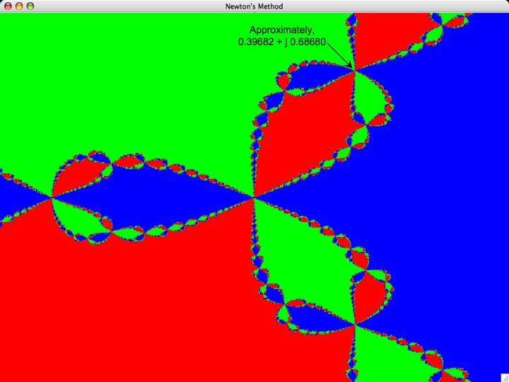
Figure 1 shows a coloring of the plane based on the application of Newton's method. Each point in the plane can be selected as an initial point. The method is applied, and the point is colored according to which of the three cube roots of unity to which the method converges. Figure 2 shows an enlargement of the region around the indicated point in the northeast of Figure 1. Notice the fractal nature of the regions of convergence.

Figure 1: Fractal Basins of Attraction for Newton's Method

Figure 2: An Enlargement of These Fractal Basins

To exhibit sensitive conditions on initial conditions, I wanted to find nearby points whose trajectory diverges under this dynamical process. Table 1 lists six points selected from Figure 2. They fall into three groups, depending on which root they converge to. I claim that one can find at least three distinct points such that each pair is as close as one wants that each converge to a seperate root.

Table 1: Limit Points for Newton's Method

Initial Guess	Limit Point
0.3899 + j 0.6871	1
0.3938 + j 0.6780	(1/2) - j (31/2)/2
0.3986 + j 0.6811	(1/2) + j (31/2)/2
0.4010 + j 0.6868	1
0.3980 + j 0.6908	(1/2) - j (31/2)/2
0.3943 + j0.6949	(1/2) + j (31/2)/2

Figure 3 and 4 display the trajectories of the six points selected for Table 1. Apparently the function is very shallow in this region. I had not realized before these explorations that these sorts of trajectories go so far from the origin before returning to converge to a root on the unit circle.

Figure 3: Real Part of Some Time Series From Newton's Method

Figure 4: Imaginary Part of Some Time Series From Newton's Method

4.0 Conclusions
Cosma provides this definition, among others, of an ergodic process:

"A ... process is ergodic when ... (almost) all trajectories generated by an ergodic process belong to a single invariant set, and they all wander from every part of that set to every other part..."

This definition is appropriate for both deterministic and stochastic processes.

The three roots of unity constitute the non-wandering (invariant) set for the dynamical system created by the above application of Newton's method. A trajectory that has converged to one of the roots does not wander to any other root. So the process is non-ergodic. Yet which root a process converges to is crucially dependent on the initial conditions. A small variation in the initial conditions leads to a long-term divergence in trajectories. This is especially evident because of the fractal structure of the basins of attraction of the three roots.

I think of the above as close to recreational mathematics. I have not tied the above example into any economics model. Common neoclassical models, such as the Arrow-Debreu model of general equilibrium, fail to tie dynamics down. I find it difficult to see how one who has absorbed this fact and understands the mathematics of dynamical systems can find credible much orthodox teaching in economics.

Why Income Inequality Leads To Recessionary Conditions

1.0 Introduction
Apparently, some have been discussing whether the gross increased inequality in the USA is connected with the depressionary conditions we are in. So I thought I would climb on my bicycle and do some arithmetic.

I take it as a stylized fact that an increase in inequality is associated with an increase in the average and marginal propensity to save.

There's something called the Harrod-Domar model of growth. I'm not sure I've ever read Domar. I've certainly read more of Harrod than I have of Domar. So in the sequel, I refer exclusively to Harrod.

Harrod defined three rates of growth: the actual rate, the warranted rate, and the natural rate. Increased inequality can result in the warranted rate exceeding the natural rate. Since the warranted rate is unstable and the actual rate cannot long exceed the natural rate, increased inequality is likely to lead to the actual rate of growth falling below and away from the warranted rate, that is, to depressions.

2.0 Harrod's Model
Harrod's model is fairly simple, but it raises deep questions.

2.1 The Actual Rate
Along a steady state growth path, the ratio, v, of the value of capital to the value of net income is constant:

v = K/Y,

where K is the value of the capital stock, and Y is the value of net income. v is known as the capital-output ratio. Thus:

dY/dt = (1/v) dK/dt

Investment, I, is defined to be the change in the value of capital with time. Hence,

(1/Y) dY/dt = (1/v) (I/Y)

The left-hand-side of of the above equation is, by definition, the rate of growth, g, of the economy. The equality of investment and savings is an accounting definition in a model with no foreign trade and no government. Therefore,

g = (1/v) (S/Y)

Define the savings rate, s:

s = S/Y

Then, a steady state growth ratio is the ratio of the savings rate to the capital-output ratio:

g = s/v

That is, the (actual) rate of growth is the quotient of the savings rate and the capital-output ratio.

2.2 The Warranted Rate
Suppose the savings rate and the capital-output ratio are as desired by income recipients (consumers) and firms, respectively. This defines Harrod's warranted rate of growth:

g_w = s_d/v_d

where the subscripts on the right hand side stand for "desired". The warranted rate of growth is being achieved when expectations are being realized and current actions are not setting up forces to disturb current expectations.

The warranted rate of growth extends Keynes' analysis to the long period. Consider the stability of a warranted growth path. If the actual rate of growth exceeds the warranted rate, capacity will be utilized at a greater rate than firms expected. They will increase investment faster than the warranted rate, and the rate of growth will deviate from the warranted rate even more. Likewise, if the actual rate falls below the warranted rate, firms will cut back on investment since the plans upon which their investment was made are not being realized. Hence, the warranted rate is unstable.

Harrod suggested that this instability of the warranted rate is more like an inverted flat-bottomed bowl than a knife-edge.

2.3 The Natural Rate
Suppose the labor force is initially fully employed. Let n be the rate of growth of the labor force:

n = (dL/dt)/L

Define the value of output produced per employed worker:

f = Y/L

Harrod-neutral technical change occurs when the value of output per worker grows at a constant rate, m, while the rate of profit stays unchanged:

m = (1/f) df/dt

Harrod-neutral technical progress implies that the productivity of labor is growing at the same rate in all industries.

Anyways, the following equation follows:

dY/dt = f dL/dt + L df/dt

Some algebra yields:

(1/Y) (dY/dt) = ( 1/L) (dL/dt) + (1/f) (df/dt)

The left hand side of the above equation is the rate of growth that keeps the labor force fully employed (or a constant percentage unemployed). Harrod calls this the natural rate of growth. Hence, assuming Harrod-neutral technological progress, the natural rate of growth is the sum of the rate of growth of the labor force and the rate of growth of labor productivity.

g_n = n + m

3.0 Conclusions
Notice that the determinants of the warranted rate of growth - the savings rate and the desired capital-output ratio - are taken as exogeneous constants. The determinants of the natural rate of growth - the growth of the labor force and Harrod-neutral technological progress - are also given. Hence, the warranted and natural rates can only be equal by a fluke.

Solow, following up on some work by Pivlin, suggested that the desired equality between the warranted and natural rates can be brought about by considering the capital-output ratio as a well-behaved function of the rate of interest. Divergences between the two rates can be corrected by variations in the distribution of income. This approach of neoclassical macroeconomics is exemplified in Solow's eponymous growth model, but it has been shown to be not well-founded in the Cambridge Capital Controversy.

If the warranted rate is below the natural rate, a moderate increase in the saving rate is desirable if the economy is exhibiting boom-like conditions. This would bring the warranted rate towards the actual rate of growth while still keeping it below the natural rate of growth.

Notice that when the warranted rate exceeds the natural rate, the economy must sometime fall below the warranted rate. The natural rate sets a limit which the economy cannot long exceed. Because of the instability of the warranted rate, such an economy will experience frequent and perhaps prolonged recessionary conditions. Since increased savings intensify the discrepancies between the warranted and natural growth rates under these conditions, increased savings intensify the frequency and severity of recessions. That is, increased inequality can intensify the frequency and severity of recessions.

References

• A. Asimakopulos (1991) Keynes's General Theory and Accumulation, Cambridge.
  1991
• Roy F. Harrod (1948) Towards a Dynamic Economics, Macmillan.
• Joan Robinson (1962) Essays in the Theory of Economic Growth, Macmillan.